scipy.stats 随机数和统计
scipy.stats 包含一些生成随机数和统计相关的工具.
随机数
stats 已经实现了两个用于封装连续随机变量和离散随机变量的通用分布类. 使用这些类已经实现了80多个连续随机变量和10个离散随机变量.
这里我们主要讨论的是连续随机变量, 当然, 这些方法几乎也都可以应用于离散随机变量.
正态分布
正态分布的方法封装在norm类中
from scipy.stats import norm
正态分布的连续随机变量的主要方法如下:
| 方法 |
描述 |
| rvs(loc=0, scale=1, size=1, random_state=None) |
随机变量(Random Variates) |
| pdf(x, loc=0, scale=1) |
概率密度函数(Probability Density Function) |
| cdf(x, loc=0, scale=1) |
累积分布函数(Cumulative Distribution Function) |
| sf(x, loc=0, scale=1) |
残存函数(Survival Function) |
| ppf(q, loc=0, scale=1) |
正态分布的累计分布函数的逆函数, 即下分位点(Percent Point Function) |
| isf(q, loc=0, scale=1) |
逆残存函数(Inverse Survival Function) |
| stats(loc=0, scale=1, moments=’mv’) |
return 均值(‘m’), 方差(‘v’), 偏度(‘s’)或峰度(‘k’) |
| fit(data, a, loc=0, scale=1) |
对一组数据进行正态分布的拟合. |
x为坐标横轴的位置, 一般用ndarry, q为概率
其他随机数
等以后用到了再补充.
百分位数
中位数是有一半值在其上一半值在其下的值, 中数也被称为百分位数50, 因为50%的观察值在它之下:
stats.scoreatpercentile(data, 50)
同样,我们也能计算百分位数90:
stats.scoreatpercentile(data, 90)
统计检验
统计检验是一个决策指示器. 例如, 如果我们有两组观察值, 我们假设他们来自于高斯过程, 我们可以用T检验来决定这两组观察值是不是显著不同:
1
2
3
4
| >>>a = np.random.normal(0, 1, size=100)
>>>b = np.random.normal(1, 1, size=10)
>>> stats.ttest_ind(a, b)
Ttest_indResult(statistic=-3.2279479468805157, pvalue=0.0016513702871169557)
|
生成的结果由以下内容组成:
- T 统计值: 一个值, 符号与两个随机过程的差异成比例, 大小与差异的程度有关.
- p 值: 两个过程相同的概率. 如果它接近1, 那么这两个过程几乎肯定是相同的. 越接近于0, 越可能这两个过程有不同的平均数.
scipy.interpolate 插值计算
scipy.interpolate 模块在拟合实验数据并估计未知点数值方面非常有用.
interpolate.interp1d(x, y)
根据给定的x轴和y轴数据返回一个拟合的function().
例如:
1
2
3
4
5
6
7
8
9
10
11
12
13
14
15
16
17
18
19
20
21
22
23
24
25
26
27
| import numpy as np
from scipy import interpolate
import matplotlib.pyplot as plt
measured_time = np.linspace(0, 1, 11)
noise = (np.random.rand(11) - 0.5) * 0.1
measures = np.sin(2 * np.pi * measured_time) + noise
linear_interp = interpolate.interp1d(measured_time, measures)
computed_time = np.linspace(0, 1, 50)
linear_results = linear_interp(computed_time)
cubic_interp = interpolate.interp1d(measured_time, measures, kind='cubic')
cubic_results = cubic_interp(computed_time)
fig, ax = plt.subplots()
plt.rcParams['axes.unicode_minus']=False
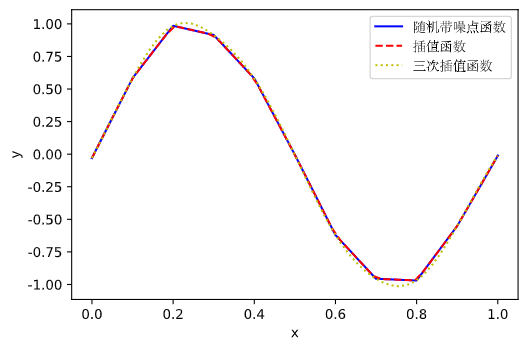
ax.plot(measured_time, measures, 'b-', label='随机函数')
ax.plot(computed_time, linear_results, 'r--', label='预测函数')
ax.plot(computed_time, cubic_results, 'y:', label='三次插值函数')
ax.legend(prop={'family' : 'STSong', 'size' : 10})
ax.set_xlabel('x')
ax.set_ylabel('y')
|
结果如图:
scipy.interpolate.interp2d 和 scipy.interpolate.interp1d 较为相似, 但是其适用对象为二维数组.
scipy.integrate 数值积分
求定积分
scipy.integrate.quad(func, a, b, args=()) 计算 $\int_a^b,func,dx$ 的结果, args为func中的参数.
这是integrate最常见的积分程序.
例如:
1
2
3
4
5
6
7
8
9
10
| >>> import numpy as np
>>> from scipy import integrate
>>> def f(x):
return np.sin(x) + np.cos(x)
>>> res, err = integrate.quad(f, 0, np.pi/2)
>>> np.allclose(res, 2)
True
>>> np.allclose(err, 0)
True
|
其他积分程序还有 fixed_quad, quadrature, romberg 等, 这里就不详细展开说了.
常微分方程(ODE)求解
scipy.integrate.solve_ivp(fun, t_span, y0, args=(), t_eval=None)
- fun: 微分方程
- t_span: t的范围
- y0: 当t=0时y的值, 为一维数组, 可以为一系列的值
- args: fun除t, y的其他参数
假设: $\frac{dy}{dt}=-2y$ , 且 $y(t=0)=1$ , 求解.
1
2
3
4
5
6
7
8
9
10
11
12
13
14
15
16
| import numpy as np
from scipy import integrate
import matplotlib.pyplot as plt
def calc_derivative(t, y):
return -2 * y
t_eval = np.linspace(0, 10, 100)
yarr = integrate.solve_ivp(calc_derivative, (0, 10), [1], t_eval=t_eval)
fig, ax = plt.subplots()
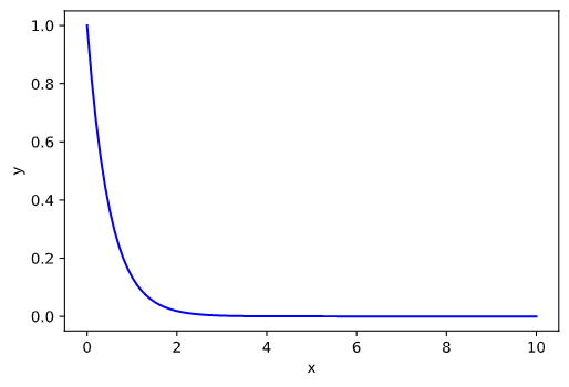
ax.plot(yarr.t, yarr.y[0], 'b-')
ax.set_xlabel('x')
ax.set_ylabel('y')
|
结果如图:
scipy.signal 信号处理
scipy.signal.detrend(data) 从信号中删除线性趋势
例如:
1
2
3
4
5
6
7
8
9
10
11
12
13
14
15
16
| import numpy as np
from scipy import signal
import matplotlib.pyplot as plt
x = np.linspace(1, 10, 100)
noise = np.random.rand(100)
y = 2 * x + noise
detrend_noice = signal.detrend(y)
fig, ax = plt.subplots()
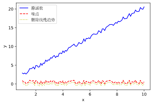
ax.plot(x, y, 'b-', label='原函数')
ax.plot(x, noise, 'r--', label='噪点')
ax.plot(x, detrend_noice, 'y:', label='删除线性趋势')
ax.legend(prop={'family' : 'STSong', 'size' : 10})
ax.set_xlabel('x')
ax.set_ylabel('y')
|
结果如图:
其他函数这里暂不讨论…
scipy.ndimage 图像处理
图像处理和分析通常被视为对二维值数组的操作. 然而, 有许多领域必须对高维图像进行分析, 医学成像和生物成像就是很好的例子. 由于其固有的多维特性, Numpy非常适合这类应用程序. scipy.ndimage 子包提供了许多常规图像处理和分析函数, 这些函数旨在与任意维数的数组一起操作. 该子包目前包括: 用于线性和非线性滤波, 二值图像形态学(binary morphology), B样条插值(B-spline interpolation)和对象测量的函数.
我暂时用不到…以后再写 其他教程
scipy.cluster 聚类分析
K-Means 聚类
k-means 算法以k为参数, 把n个对象分成k个簇, 使簇内具有较高的相似度, 而簇间的相似度较低.
- 随机选择k个点作为初始的聚类中心.
- 对于剩下的点, 根据其与聚类中心的距离, 将其归入最近的簇.
- 对每个簇, 计算所有点的均值作为新的聚类中心.
- 重复2, 3直到聚类中心不再发生改变.
有下面例子:
1
2
3
4
5
6
7
8
9
10
11
12
13
14
15
16
17
18
19
20
21
22
23
24
25
26
| import numpy as np
from scipy import cluster
import matplotlib.pyplot as plt
data = np.vstack((np.random.rand(20,2) + np.array([.5,.5]), np.random.rand(20,2)))
np.random.shuffle(data)
data_whitened = cluster.vq.whiten(data)
centroids, _ = cluster.vq.kmeans(data_whitened, 3)
clx, _ = cluster.vq.vq(data_whitened, centroids)
fig, ax = plt.subplots()
clx_0 = data_whitened[np.where(clx == 0)]
clx_1 = data_whitened[np.where(clx == 1)]
clx_2 = data_whitened[np.where(clx == 2)]
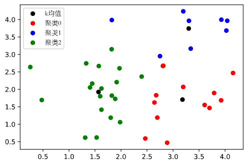
ax.scatter(centroids[:, 0], centroids[:, 1], c='k', label="k均值")
ax.scatter(clx_0[:, 0], clx_0[:, 1], c='r', label="聚类0")
ax.scatter(clx_1[:, 0], clx_1[:, 1], c='b', label="聚类1")
ax.scatter(clx_2[:, 0], clx_2[:, 1], c='g', label="聚类2")
ax.legend(prop={'family' : 'STSong', 'size' : 10})
|
结果如图:
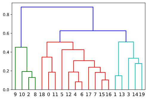
Hierarchical 聚类
层次聚类方法对给定的数据集进行层次的分解, 直到某种条件满足为止.
在已经得到距离值之后, 元素间可以被联系起来. 通过分离和融合可以构建一个结构. 传统上, 表示的方法是树形数据结构, 层次聚类算法, 要么是自底向上聚集型的, 即从叶子节点开始, 最终汇聚到根节点; 要么是自顶向下分裂型的, 即从根节点开始, 递归的向下分裂.
实例如下:
1
2
3
4
5
6
7
8
9
10
11
12
13
14
15
16
| import numpy as np
from scipy import cluster
import matplotlib.pyplot as plt
data = np.vstack((np.random.rand(10,2) + np.array([.5,.5]), np.random.rand(10,2)))
np.random.shuffle(data)
data_dis = cluster.hierarchy.distance.pdist(data, 'euclidean')
hierarchical_cluster = cluster.hierarchy.linkage(data_dis,method='average')
p = cluster.hierarchy.dendrogram(Z)
|
输出结果如图:
参考文献
1. SciPy — SciPy v1.4.1 Reference Guide
2. Varoquaux, Gaël, et al. Scipy Lecture Notes. 2015.